Basic care and feeding of data in R
Buckle your seatbelt
Ignore if you don't need this bit of support.
Now is the time to make sure you are working in an appropriate directory on your computer, probably through the use of an RStudio Project. Enter getwd() in the Console to see current working directory or, in RStudio, this is displayed in the bar at the top of Console.
You should clean out your workspace. In RStudio, click on the "Clear" broom icon from the Environment tab or use Session > Clear Workspace. You can also enter rm(list = ls()) in the Console to accomplish same.
Now restart R. This will ensure you don't have any packages loaded from previous calls to library(). In RStudio, use Session > Restart R. Otherwise, quit R with q() and re-launch it.
Why do we do this? So that the code you write is complete and re-runnable. If you return to a clean slate often, you will root out hidden dependencies where one snippet of code only works because it relies on objects created by code saved elsewhere or, much worse, never saved at all. Similarly, an aggressive clean slate approach will expose any usage of packages that have not been explicitly loaded.
Finally, open a new R script and develop and run your code from there. In RStudio, use File > New File > R Script. Save this script with a name ending in .r or .R, containing no spaces or other funny stuff, and that evokes whatever it is we're doing today. Example: cm004_data-care-feeding.r.
Get the Gapminder data
We will work with some of the data from the Gapminder project. I've released this as an R package, so we can install it from CRAN like so:
install.packages("gapminder")
Now load the package:
library(gapminder)
Meet your first data.frame
Whenever you have rectangular, spreadsheet-y data, your default data receptacle in R is a data.frame. Do not depart from this without good reason. data.frames are awesome because...
- data.frames package related variables neatly together,
- keeping them in sync vis-a-vis row order
- applying any filtering of observations uniformly
- most functions for inference, modelling, and graphing are happy to be passed a data.frame via a
data =argument as the place to find the variables you're working on; the latest and greatest packages actually require that your data be in a data.frame - data.frames -- unlike general arrays or, specifically, matrices in R -- can hold variables of different flavors (heuristic term defined later), such as character data (subject ID or name), quantitative data (white blood cell count), and categorical information (treated vs. untreated)
By loading the gapminder package, we now have access to a data.frame by the same name. Get an overview of this with str(), which displays the structure of an object. It will provide a sensible description of almost anything and, worst case, nothing bad can actually happen. When in doubt, just str() some of the recently created objects to get some ideas about what to do next.
str(gapminder)
## 'data.frame':    1704 obs. of  6 variables:
##  $ country  : Factor w/ 142 levels "Afghanistan",..: 1 1 1 1 1 1 1 1 1 1 ...
##  $ continent: Factor w/ 5 levels "Africa","Americas",..: 3 3 3 3 3 3 3 3 3 3 ...
##  $ year     : num  1952 1957 1962 1967 1972 ...
##  $ lifeExp  : num  28.8 30.3 32 34 36.1 ...
##  $ pop      : num  8425333 9240934 10267083 11537966 13079460 ...
##  $ gdpPercap: num  779 821 853 836 740 ...
We could print the whole thing to screen (not so useful with datasets of any size) but it's nicer to look at the first bit or the last bit or a random snippet.
head(gapminder)
##       country continent year lifeExp      pop gdpPercap
## 1 Afghanistan      Asia 1952  28.801  8425333  779.4453
## 2 Afghanistan      Asia 1957  30.332  9240934  820.8530
## 3 Afghanistan      Asia 1962  31.997 10267083  853.1007
## 4 Afghanistan      Asia 1967  34.020 11537966  836.1971
## 5 Afghanistan      Asia 1972  36.088 13079460  739.9811
## 6 Afghanistan      Asia 1977  38.438 14880372  786.1134
tail(gapminder)
##       country continent year lifeExp      pop gdpPercap
## 1699 Zimbabwe    Africa 1982  60.363  7636524  788.8550
## 1700 Zimbabwe    Africa 1987  62.351  9216418  706.1573
## 1701 Zimbabwe    Africa 1992  60.377 10704340  693.4208
## 1702 Zimbabwe    Africa 1997  46.809 11404948  792.4500
## 1703 Zimbabwe    Africa 2002  39.989 11926563  672.0386
## 1704 Zimbabwe    Africa 2007  43.487 12311143  469.7093
gapminder[sample(nrow(gapminder), 10), ]
##               country continent year lifeExp        pop gdpPercap
## 125             Benin    Africa 1972  47.014    2761407  1085.797
## 1458        Swaziland    Africa 1977  52.537     551425  3781.411
## 648             Haiti  Americas 2007  60.916    8502814  1201.637
## 471       El Salvador  Americas 1962  52.307    2747687  3776.804
## 834  Korea, Dem. Rep.      Asia 1977  67.159   16325320  4106.301
## 296             China      Asia 1987  67.274 1084035000  1378.904
## 1097      New Zealand   Oceania 1972  71.890    2929100 16046.037
## 803             Japan      Asia 2002  82.000  127065841 28604.592
## 1441            Sudan    Africa 1952  38.635    8504667  1615.991
## 1444            Sudan    Africa 1967  42.858   12716129  1687.998
More ways to query basic info on a data.frame. Note: with some of the commands below we're benefiting from the fact that even though data.frames are technically NOT matrices, it's usually fine to think of them that way and many functions have reasonable methods for both types of input.
names(gapminder)
## [1] "country"   "continent" "year"      "lifeExp"   "pop"       "gdpPercap"
ncol(gapminder)
## [1] 6
length(gapminder)
## [1] 6
head(rownames(gapminder))
## [1] "1" "2" "3" "4" "5" "6"
dim(gapminder)
## [1] 1704    6
nrow(gapminder)
## [1] 1704
#dimnames(gapminder) # ill-advised here ... too many rows
A statistical overview can be obtained with summary()
summary(gapminder)
##         country        continent        year         lifeExp
##  Afghanistan:  12   Africa  :624   Min.   :1952   Min.   :23.60
##  Albania    :  12   Americas:300   1st Qu.:1966   1st Qu.:48.20
##  Algeria    :  12   Asia    :396   Median :1980   Median :60.71
##  Angola     :  12   Europe  :360   Mean   :1980   Mean   :59.47
##  Argentina  :  12   Oceania : 24   3rd Qu.:1993   3rd Qu.:70.85
##  Australia  :  12                  Max.   :2007   Max.   :82.60
##  (Other)    :1632
##       pop              gdpPercap
##  Min.   :6.001e+04   Min.   :   241.2
##  1st Qu.:2.794e+06   1st Qu.:  1202.1
##  Median :7.024e+06   Median :  3531.8
##  Mean   :2.960e+07   Mean   :  7215.3
##  3rd Qu.:1.959e+07   3rd Qu.:  9325.5
##  Max.   :1.319e+09   Max.   :113523.1
##
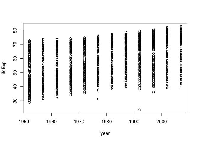
Although we haven't begun our formal coverage of visualization yet, it's so important for smell-testing dataset that we will make a few figures anyway. Here we use only base R graphics, which are very basic.
plot(lifeExp ~ year, gapminder)
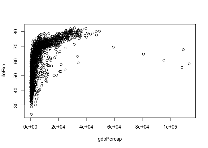
plot(lifeExp ~ gdpPercap, gapminder)
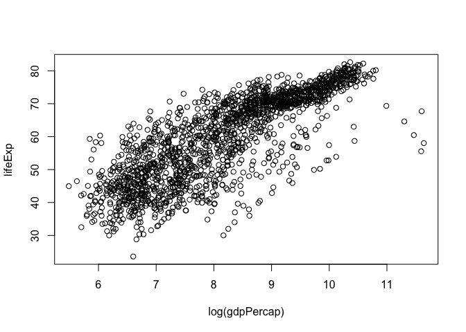
plot(lifeExp ~ log(gdpPercap), gapminder)
Let's go back to the result of str() to talk about data.frames and vectors in R
str(gapminder)
## 'data.frame':    1704 obs. of  6 variables:
##  $ country  : Factor w/ 142 levels "Afghanistan",..: 1 1 1 1 1 1 1 1 1 1 ...
##  $ continent: Factor w/ 5 levels "Africa","Americas",..: 3 3 3 3 3 3 3 3 3 3 ...
##  $ year     : num  1952 1957 1962 1967 1972 ...
##  $ lifeExp  : num  28.8 30.3 32 34 36.1 ...
##  $ pop      : num  8425333 9240934 10267083 11537966 13079460 ...
##  $ gdpPercap: num  779 821 853 836 740 ...
A data.frame is a special case of a list, which is used in R to hold just about anything. data.frames are the special case where the length of each list component is the same. data.frames are superior to matrices in R because they can hold vectors of different flavors (heuristic term explained below), e.g. numeric, character, and categorical data can be stored together. This comes up alot.
Look at the variables inside a data.frame
To specify a single variable from a data.frame, use the dollar sign $. Let's explore the numeric variable for life expectancy.
head(gapminder$lifeExp)
## [1] 28.801 30.332 31.997 34.020 36.088 38.438
summary(gapminder$lifeExp)
##    Min. 1st Qu.  Median    Mean 3rd Qu.    Max.
##   23.60   48.20   60.71   59.47   70.85   82.60
hist(gapminder$lifeExp)

The year variable is a numeric integer variable, but since there are so few unique values it also functions a bit like a categorical variable.
summary(gapminder$year)
##    Min. 1st Qu.  Median    Mean 3rd Qu.    Max.
##    1952    1966    1980    1980    1993    2007
table(gapminder$year)
##
## 1952 1957 1962 1967 1972 1977 1982 1987 1992 1997 2002 2007
##  142  142  142  142  142  142  142  142  142  142  142  142
The variables for country and continent hold truly categorical information, which is stored as a factor in R.
class(gapminder$continent)
## [1] "factor"
summary(gapminder$continent)
##   Africa Americas     Asia   Europe  Oceania
##      624      300      396      360       24
levels(gapminder$continent)
## [1] "Africa"   "Americas" "Asia"     "Europe"   "Oceania"
nlevels(gapminder$continent)
## [1] 5
The levels of the factor continent are "Africa", "Americas", etc. and this is what's usually presented to your eyeballs by R. In general, the levels are friendly human-readable character strings, like "male/female" and "control/treated". But never ever ever forget that, under the hood, R is really storing integer codes 1, 2, 3, etc. Look at the result from str(gapminder$continent) if you are skeptical.
str(gapminder$continent)
##  Factor w/ 5 levels "Africa","Americas",..: 3 3 3 3 3 3 3 3 3 3 ...
This Janus-like nature of factors means they are rich with booby traps for the unsuspecting but they are a necessary evil. I recommend you resolve to learn how to properly care and feed for factors. The pros far outweigh the cons. Specifically in modelling and figure-making, factors are anticipated and accommodated by the functions and packages you will want to exploit.
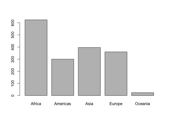
Here we count how many observations are associated with each continent and, as usual, try to portray that info visually. This makes it much easier to quickly see that African countries are well represented in this dataset.
table(gapminder$continent)
##
##   Africa Americas     Asia   Europe  Oceania
##      624      300      396      360       24
barplot(table(gapminder$continent))
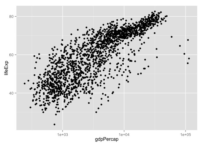
In the figures below, we see how factors can be put to work in figures. The continent factor is easily mapped into "facets" or colors and a legend by the ggplot2 package. Making figures with ggplot2 is covered elsewhere so feel free to just sit back and enjoy these plots or blindly copy/paste.
## install ggplot2 if you don't have it!
## install.packages("ggplot2")
library(ggplot2)
p <- ggplot(subset(gapminder, continent != "Oceania"),
aes(x = gdpPercap, y = lifeExp)) # just initializes
p <- p + scale_x_log10() # log the x axis the right way
p + geom_point() # scatterplot
p + geom_point(aes(color = continent)) # map continent to color
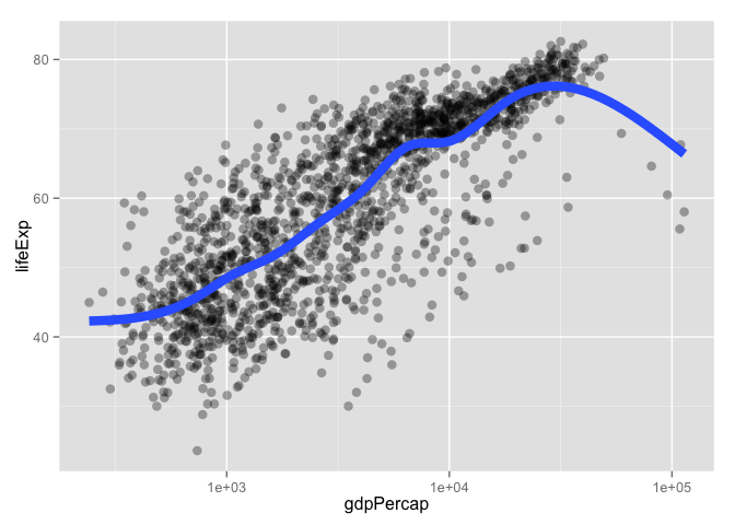
p + geom_point(alpha = (1/3), size = 3) + geom_smooth(lwd = 3, se = FALSE)
## geom_smooth: method="auto" and size of largest group is >=1000, so using gam with formula: y ~ s(x, bs = "cs"). Use 'method = x' to change the smoothing method.
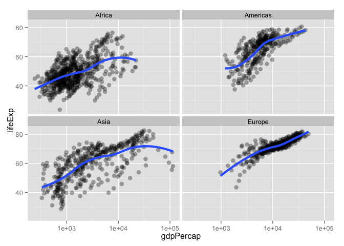
p + geom_point(alpha = (1/3), size = 3) + facet_wrap(~ continent) +
geom_smooth(lwd = 1.5, se = FALSE)
## geom_smooth: method="auto" and size of largest group is <1000, so using loess. Use 'method = x' to change the smoothing method.
## geom_smooth: method="auto" and size of largest group is <1000, so using loess. Use 'method = x' to change the smoothing method.
## geom_smooth: method="auto" and size of largest group is <1000, so using loess. Use 'method = x' to change the smoothing method.
## geom_smooth: method="auto" and size of largest group is <1000, so using loess. Use 'method = x' to change the smoothing method.

subset() is a nice way to isolate bits of data.frames (and other things)
Logical little pieces of data.frames are useful for sanity checking, prototyping visualizations or computations for later scale-up, etc. Many functions are happy to restrict their operations to a subset of observations via a formal subset = argument. There is a stand-alone function, also confusingly called subset(), that can isolate pieces of an object for inspection or assignment. Although subset() can work on objects other than data.frames, we focus on that usage here.
The subset() function has a subset = argument (sorry, not my fault it's so confusing) for specifying which observations to keep. This expression will be evaluated within the specified data.frame, which is non-standard but convenient.
subset(gapminder, subset = country == "Uruguay")
##      country continent year lifeExp     pop gdpPercap
## 1621 Uruguay  Americas 1952  66.071 2252965  5716.767
## 1622 Uruguay  Americas 1957  67.044 2424959  6150.773
## 1623 Uruguay  Americas 1962  68.253 2598466  5603.358
## 1624 Uruguay  Americas 1967  68.468 2748579  5444.620
## 1625 Uruguay  Americas 1972  68.673 2829526  5703.409
## 1626 Uruguay  Americas 1977  69.481 2873520  6504.340
## 1627 Uruguay  Americas 1982  70.805 2953997  6920.223
## 1628 Uruguay  Americas 1987  71.918 3045153  7452.399
## 1629 Uruguay  Americas 1992  72.752 3149262  8137.005
## 1630 Uruguay  Americas 1997  74.223 3262838  9230.241
## 1631 Uruguay  Americas 2002  75.307 3363085  7727.002
## 1632 Uruguay  Americas 2007  76.384 3447496 10611.463
Contrast the above command with this one accomplishing the same thing:
gapminder[1621:1632, ]
##      country continent year lifeExp     pop gdpPercap
## 1621 Uruguay  Americas 1952  66.071 2252965  5716.767
## 1622 Uruguay  Americas 1957  67.044 2424959  6150.773
## 1623 Uruguay  Americas 1962  68.253 2598466  5603.358
## 1624 Uruguay  Americas 1967  68.468 2748579  5444.620
## 1625 Uruguay  Americas 1972  68.673 2829526  5703.409
## 1626 Uruguay  Americas 1977  69.481 2873520  6504.340
## 1627 Uruguay  Americas 1982  70.805 2953997  6920.223
## 1628 Uruguay  Americas 1987  71.918 3045153  7452.399
## 1629 Uruguay  Americas 1992  72.752 3149262  8137.005
## 1630 Uruguay  Americas 1997  74.223 3262838  9230.241
## 1631 Uruguay  Americas 2002  75.307 3363085  7727.002
## 1632 Uruguay  Americas 2007  76.384 3447496 10611.463
Yes, these both return the same result. But the second command is horrible for these reasons:
- It contains Magic Numbers). The reason for keeping rows 1621 to 1632 will be non-obvious to someone else and that includes you in a couple of weeks.
- It is fragile. If the rows of
gapminderare reordered or if some observations are eliminated, these rows may no longer correspond to the Uruguay data.
In contrast, the first command, using subset(), is self-documenting; one does not need to be an R expert to take a pretty good guess at what's happening. It's also more robust. It will still produce the correct result even if gapminder has undergone some reasonable set of transformations.
The subset() function can also be used to select certain variables via the select argument. It also offers unusual flexibility, so you can, for example, provide the names of variables you wish to keep without surrounding by quotes. I suppose this is mostly a good thing, but even the documentation stresses that the subset() function is intended for interactive use (which I interpret more broadly to mean data analysis, as opposed to programming).
You can use subset = and select = together to simultaneously filter rows and columns or variables.
subset(gapminder, subset = country == "Mexico",
       select = c(country, year, lifeExp))
##     country year lifeExp
## 985  Mexico 1952  50.789
## 986  Mexico 1957  55.190
## 987  Mexico 1962  58.299
## 988  Mexico 1967  60.110
## 989  Mexico 1972  62.361
## 990  Mexico 1977  65.032
## 991  Mexico 1982  67.405
## 992  Mexico 1987  69.498
## 993  Mexico 1992  71.455
## 994  Mexico 1997  73.670
## 995  Mexico 2002  74.902
## 996  Mexico 2007  76.195
Many of the functions for inference, modelling, and graphics that permit you to specify a data.frame via data = also offer a subset = argument that limits the computation to certain observations. Here's an example of subsetting the data to make a plot just for Colombia and a similar call to lm for fitting a linear model to just the data from Colombia.
p <- ggplot(subset(gapminder, country == "Colombia"),
            aes(x = year, y = lifeExp))
p + geom_point() + geom_smooth(lwd = 1, se = FALSE, method = "lm")

(minYear <- min(gapminder$year))
## [1] 1952
myFit <- lm(lifeExp ~ I(year - minYear), gapminder,
            subset = country == "Colombia")
summary(myFit)
##
## Call:
## lm(formula = lifeExp ~ I(year - minYear), data = gapminder, subset = country ==
##     "Colombia")
##
## Residuals:
##     Min      1Q  Median      3Q     Max
## -2.7841 -0.3816  0.1840  0.8413  1.8034
##
## Coefficients:
##                   Estimate Std. Error t value Pr(>|t|)
## (Intercept)       53.42712    0.71223   75.01 4.33e-15 ***
## I(year - minYear)  0.38075    0.02194   17.36 8.54e-09 ***
## ---
## Signif. codes:  0 '***' 0.001 '**' 0.01 '*' 0.05 '.' 0.1 ' ' 1
##
## Residual standard error: 1.312 on 10 degrees of freedom
## Multiple R-squared:  0.9679,    Adjusted R-squared:  0.9647
## F-statistic: 301.3 on 1 and 10 DF,  p-value: 8.537e-09
Review of data.frames and the best ways to exploit them
Use data.frames!!!
The most modern, slick way to work with data.frame is with the dplyr package. We will cover this extensively in the coming weeks. Here's material for 2014, though these will likely get an update:
- Introduction to dplyr
dplyrfunctions for a single dataset- Cheatsheet for
dplyrjoins, i.e. "two table" operations
Work within your data.frames by passing them to the data = argument of functions that offer that. If you need to restrict operations, use the subset = argument. Do computations or make figures in situ -- don't create little copies and excerpts of your data. This will leave a cleaner workspace and cleaner code.
This workstyle leaves behind code that is also fairly self-documenting, e.g.,
lm(lifeExp ~ year, gapminder, subset = country == "Colombia")
plot(lifeExp ~ year, gapminder, subset = country == "Colombia")
The availability and handling of data = and subset = arguments is broad enough-- though sadly not universal -- that sometimes you can even copy and paste these argument specifications, for example, from an exploratory plotting command into a model-fitting command. Consistent use of this convention also makes you faster at writing and reading such code.
Two important practices
- give variables short informative names (
lifeExpversus "X5") - refer to variables by name, not by column number
This will produce code that is self-documenting and more robust. Variable names often propagate to downstream outputs like figures and numerical tables and therefore good names have a positive multiplier effect throughout an analysis.
If a function doesn't have a data = argument where you can provide a data.frame, you can fake it with with(). with() helps you avoid the creation of temporary, confusing little partial copies of your data. Use it -- possibly in combination with subset() -- to do specific computations without creating all the intermediate temporary objects you have no lasting interest in. with() is also useful if you are tempted to use attach() in order to save some typing. Never ever use attach(). It is evil. If you've never heard of it, consider yourself lucky.
Example: How would you compute the correlation of life expectancy and GDP per capita for the country of Colombia? The cor() function sadly does not offer the usual data = and subset = arguments. Here's a nice way to combine with() and subset() to accomplish without unnecessary object creation and with fairly readable code.
with(subset(gapminder, subset = country == "Colombia"),
     cor(lifeExp, gdpPercap))
## [1] 0.9514699